This article continues the series about approximating circles using Bézier curves. Preceding parts analysed linear and quadratic curves. This entry examines cubic Bézier curves. It presents a construction of a spline which approximates a circle and derives practical formulæ based on different optimisation criteria. Table of Contents
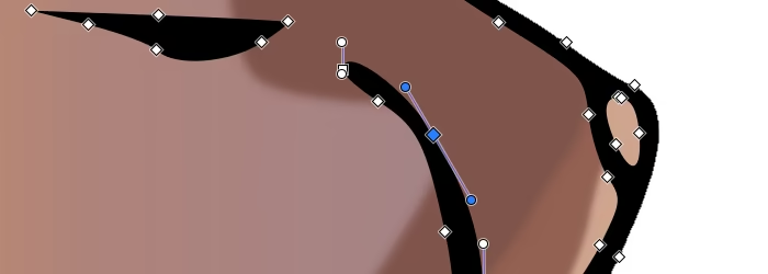 Fig. 1 Inkscape highlighting a joint (a blue diamond) and adjacent control points (blue circles).
Cubic Bézier curves are available in many popular tools. They are widely used in vector graphics editing and animation software, and provide flexibility while remaining intuitive to edit. For example, Fig. 1 presents Inkscape’s Node Tool highlighting a joint and two control points adjacent to it. Dragging the points offers a user-friendly way to modify the shape.
A cubic Bézier curve uses four control points: \(\def\P{\mathbf P}\P_0\) through \(\P_3\) and is defined by the following parametric function: $$\def\tau2k{\frac τ{2k}} \def\D{Δ\mathbf P} \def\O{\mathbf O} \def\R2{\mathtt{R2}} \def\V{\mathbf V} \def\VR{\mathbf V^⟂} \def\argmin{\operatorname*{arg\,min}} \def\lerp{\operatorname{lerp}} B(t)=(1-t)^3\P_0 + 3(1-t)^2t\P_1 + 3(1-t)t^2\P_2 + t^3\P_3$$
Drawing a circle
A \(k\)-segment cubic Bézier spline (i.e. \(k\) curves joined end-to-end) uses \(3k+1\) control points (two joints and two control handles per segment with adjacent curves sharing a joint). Compared to a quadratic Bézier spline, this introduces an additional handle per segment, offering more degrees of freedom in shaping the path. Fig. 2 shows how an approximation of a circle with three free parameters \(r\), \(h\) and \(g\) is constructed.$$\begin{align} \V_i &= \left(\phantom-\cos\frac{iτ}k, \sin\frac{iτ}k\right)\\ \VR_i &= \left(-\sin\frac{iτ}k, \cos\frac{iτ}k\right)\\[1em] \P_0 &= \phantom{g(}r\V_0\\ \P_1 &= g(r\V_0 + h\VR_0)\\ \P_2 &= g(r\V_1 - h\VR_1)\\ \P_3 &= \phantom{g(}r\V_1\\ &\ \ \vdots\\ \P_{3i-1} &= g(r\V_i - h\VR_i)\\ \P_{3i\phantom{+0}} &= \phantom{g(}r\V_i\\ \P_{3i+1} &= g(r\V_i + h\VR_i)\\ &\ \ \vdots \end{align}$$
The formulæ use two families of vectors. \(\V_i\) are unit vectors evenly spaced in direction around a circle. They define the direction towards the corresponding anchor points \(\P_{3i}\). \(\VR_i\) are those vectors rotated 90°. For example, \(\V_1\) describes direction of the \(\overline{\O\P_3}\) line (where \(\O\) is the origin) and \(\VR_1\) describes direction of the tangent line at \(\P_3\).
The placement of the control points is defined using those vector families: \(r\V_i\) produces joints evenly spaced around a circle of radius \(r\) and \(r\V_i±h\VR_i\) produces handles on a tangent line \(h\) units away from the joints. The parameter \(g\) moves the handles in a straight line closer or further away from the origin.
With \(g=1\) those handles lie directly on the tangent lines such that a joint and its two adjacent handles are collinear resulting in a \(C^1\) continuous shape. With the remaining two degrees of freedom, the \(r\) and \(h\) parameters, it’s furthermore possible to create an approximation of a circle which is \(C^2\) continuous. The condition for that is \(h = r\sin\tau2k/(2 + \cos\tau2k)\); for derivation of the formula see appendix II. However (analogous to the quadratic spline), enforcing \(C^3\) continuity results in the entire spline being fully determined by the first four points.
The complexity of the optimisation problem — caused by the combination of three degrees of freedom and high degree of the curve’s polynomial — necessitates the use of numerical methods and symbolic manipulation to find the optimal parameters. \(C^2\) and \(C^1\) continuous splines are constrained enough that closed-form formulæ for the parameters are attainable (see appendix III), but a solution for a \(C^0\) continuous spline is too complex to tackle analytically, so this article resorts to tabulating the best numerical solutions found (see appendix IV).
To approximate a circle of radius \(R\) by \(k\) cubic Bézier curves, the curves are joined to form a cubic Bézier spline with the following \(3k+1\) control points from \(\P_0\) to \(P_{3k}\): $$\begin{align} \P_i &=\begin{cases} \phantom{g(}r\V_j &\quad\text{if } i = 3j\\ g(r\V_j ± h\VR_j) &\quad\text{if } i = 3j±1\\ \end{cases}\\ &\hspace{-1.25em}\text{where:}\\ \V_j &=\left(\phantom-R\cos\frac{jτ}k, R\sin\frac{jτ}k\right)\\ \VR_j&=\left( -R\sin\frac{jτ}k, R\cos\frac{jτ}k\right)\\ \end{align}$$
With \(\P_0=\P_{3k}\), the spline forms a closed shape. The \(r\), \(h\) and \(g\) parameters determine how well the spline approximates a circle and are chosen depending on the requirements on the shape’s continuity. \(C^0\) continuous shape allows for the lowest maximum absolute drift, but applications such as animation or simulation may require \(C^1\) or \(C^2\) continuity.
Values for all those cases as well as direct formulæ for the special case of a four-segment spline are listed below:
With nine segments the \(C^1\) and \(C^0\) continuous approximations reach a maximum absolute drift of less than one in a million as shown in Fig. 3. Better tuning of the numeric optimisation algorithms could refine the parameters for \(C^0\) continuous cubic Bézier splines further. Nevertheless, it’s unclear that more accurate approximations, especially at high number of segments, are necessary in practice.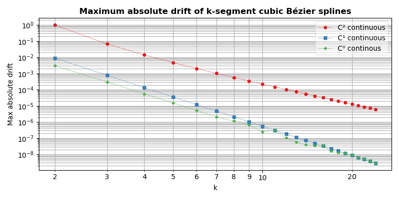 Fig. 3 Comparison of maximum absolute drift of cubic Bézier splines with different number of segments and methods of picking their parameters. (Click to open the image).
To visually compare different ways of approximating a circle, Fig. 4 offers an interactive demonstration using the cubic splines described in this article, as well as the quadratic and linear splines from previous articles in the series.Fig. 4 Interactive demonstration of different methods of drawing a circle with cubic, quadratic and linear Bézier splines. Requires JavaScript to function.
Appendix
The subsequent sections contain the detailed mathematical proofs and computational methods that underpin the results discussed in the main text of the article above. These include the derivations for general curve derivatives (§I) and shape continuity constraints (§II), as well as the optimisation logic used to calculate the ideal parameters for cubic Bézier splines (§III and §IV) with the help of SymPy, a symbolic manipulation library, and SciPy, a numeric optimisation library.
I Derivatives of Bézier curves
The previous article looked at the special case of derivatives of quadratic Bézier curves and observed that they were curves of a lower order. This holds for the general case.3 Let \(B^n(\P_0,…,\P_n;t)\) denote a Bézier curve of order \(n\) with given control points, then for positive \(n\): $${B^n}'(\P_0,…,\P_n;t) = nB^{n-1}(\D_0,…,\D_{n-1};t)$$
where \(\D_i=\P_{i+1}-\P_{i}\). The de Casteljau algorithm2 yields a recursive definition of the curve: $$\begin{align} B^0(\P_0; t) &≡\P_0\\ B^n(\P_0,…,\P_n;t) &=(1-t)B^{n-1}(\P_0,…,\P_{n-1};t)\\ &{}+tB^{n-1}(\P_1,…,\P_n;t) \end{align}$$
By the chain rule, \({B^1}'(\P_0, \P_1; t) = -\P_0+\P_1 = 1·B^0(\D_0;t)\) which proves the base case. This leaves the induction step: $$\begin{split} &{B^n}'(\P_0,…,\P_n;t)\\ &\quad{}=\frac d{dt}\bigl((1-t)B^{n-1}(\P_0,…,\P_{n-1};t) + tB^{n-1}(\P_1,…,\P_n;t)\bigr)\\ &\quad{}=-B^{n-1}(\P_0,…,\P_{n-1};t) + B^{n-1}(\P_1,…,\P_n;t)\\ &\quad{}+(1-t){B^{n-1}}'(\P_0,…,\P_{n-1};t) +t{B^{n-1}}'(\P_1,…,\P_n;t)\\ \end{split}$$
By linearity of the Bézier curve, the first line is simplified to a single curve function: $$\begin{split} &-B^{n-1}(\P_0,…,\P_{n-1};t) + B^{n-1}(\P_1,…,\P_n;t)\\ &\quad{}=B^{n-1}(\P_1-\P_0,…,\P_n-\P_{n-1};t)\\ &\quad{}=B^{n-1}(\D_0,…,\D_{n-1};t) \end{split}$$
The second line is transformed by applying the induction hypothesis and then combined using the recursive definition of the curve: $$\begin{split} &(1-t){B^{n-1}}'(\P_0,…,\P_{n-1};t) + t{B^{n-1}}'(\P_1,…,\P_n;t)\\ &\quad{}=(n-1)(1-t)B^{n-2}(\D_0,…,\D_{n-2};t)\\ &\quad{}+(n-1)tB^{n-2}(\D_1,…,\D_{n-1};t)\\ &\quad{}=(n-1)B^{n-1}(\D_0,…,\D_{n-1};t) \end{split}$$
Substituting those results into the formula: $$\begin{split} &{B^n}'(\P_0,…,\P_n;t)\\ &\quad{}=B^{n-1}(\D_0,…,\D_{n-1};t)\\ &\quad{}+(n-1)B^{n-1}(\D_0,…,\D_{n-1};t)\\ &\quad{}=nB^{n-1}(\D_0,…,\D_{n-1};t) \end{split}$$
QED.
II Continuity of Bézier splines
As previously discussed, a \(C^m\) continuity requires first \(m\) derivatives of the curve to be continuous.4 The general equation for a derivative of a Bézier curve enables easy analysis of the continuity conditions of Bézier splines. For \(C^1\) continuity, the first derivative must be continuous. Let \(P_0\) through \(P_{2n}\) denote a two-segment Bézier spline of order \(n\): $$\begin{align} {B^n}'(\P_0,…,\P_n;0) &= n(\P_1-\P_0)\\ {B^n}'(\P_0,…,\P_n;1) &= n(\P_n - \P_{n-1})\\ {B^n}'(\P_0,…,\P_n;1) &= {B^n}'(\P_n,…,\P_{2n};0)\\ \P_n-\P_{n-1} &= \P_{n+1}-\P_n\\ \P_{n+1} &= 2\P_n - \P_{n-1}\\[.5em] \end{align}$$
Applying this result to the approximation of a circle constructed in Fig. 2 a constraint on one of the parameters is derived: $$\begin{align} \P_4 &= 2\P_3 - \P_{2}\\ g(r\V_1 + h\VR_1) &= 2r\V_1 - g(r\V_1 - h\VR_1)\\ 2gr\V_1 &= 2r\V_1\\ g &= 1 \end{align}$$
For \(C^2\) continuity, the second derivative must be continuous: $$\begin{align} {B^n}''(\P_0,…,\P_n;t) &= n{B^{n-1}}'(\D_0,…,\D_{n-1};t)\\[.5em] {B^n}''(\P_0,…,\P_n;1) &= {B^n}''(\P_n,…,\P_{2n};0)\\ n(\D_{n-1}-\D_{n-2}) &= n(\D_{n+1}-\D_n)\\ (\P_n-\P_{n-1})-(\P_{n-1}-\P_{n-2}) &= (\P_{n+2}-\P_{n+1})-(\P_{n+1}-\P_n)\\ \P_n-2\P_{n-1}+\P_{n-2} &= \P_{n+2}-2\P_{n+1}+\P_n\\ -2\P_{n-1}+\P_{n-2} &= \P_{n+2}-4\P_n + 2\P_{n-1}\\ \P_{n+2} &= \P_{n-2} + 4(\P_n - \P_{n-1})\\ \end{align}$$
Applying this and the \(g=1\) constraint to the points in the approximation of a circle yields: $$\begin{align} \P_5 &= \P_1 + 4(\P_3 - \P_2)\\ r\V_2 - h\VR_2 &= r\V_0 + h\VR_0 + 4(r\V_1 - r\V_1 + h\VR_1)\\ r\V_2 - h\VR_2 &= r\V_0 + h\VR_0 + 4h\VR_1\\ h(\VR_0 + 4\VR_1 + \VR_2) &= r(\V_2 - \V_0) \\ \end{align}$$
Let \(Φ=τ/k\); looking at the x coordinate it follows: $$\begin{align} h(0 - 4\sin Φ - \sin 2Φ) &= r(\cos 2Φ - 1) \\ h(-4\sin Φ - 2\sin Φ\cos Φ) &= r(1 - 2\sin^2 Φ - 1) \\ -2h\sin Φ(2 + \cos Φ) &= -2r\sin^2 Φ \\ h &= \frac{r\sin Φ}{2 + \cos Φ}\\ \end{align}$$
Analogous to the previous investigation around quadratic splines, requiring a cubic spline to be \(C^3\) continuous removes any degrees of freedom for all but the first segment in the spline. It’s therefore impossible to reasonably approximate a circle with a \(C^3\) continuous cubic Bézier spline. Meanwhile, constraints for \(C^1\) and \(C^2\) continuity are as follows:
$$\begin{align} \text{$C^1$ continuity:}&\quad g=1\\ \text{$C^2$ continuity:}&\quad h=\frac{r\sin(τ/k)}{2 + \cos(τ/k)} \end{align}$$
III Optimising \(C^2\) and \(C^1\) continuous splines
Optimising a \(C^2\) continuous \(k\)-segment cubic Bézier spline, means searching for \((r_2, h_2, g_2)\) parameters which result in the lowest maximum absolute drift. By the symmetry of the spline, it’s enough to look at only one segment whose control points are placed symmetrically about the horizontal axis. For brevity, let \(C=\cos\tau2k\) and \(S=\sin\tau2k\): $$\begin{align} (x_0, y_0) &= (rC, rS) & (x_1, y_1) &= (grC + ghS, grS - ghC)\\ \P_0 &= (x_0, \phantom-y_0) & \P_1 &= (x_1, \phantom-y_1)\\ \P_3 &= (x_0, -y_0) & \P_2 &= (x_1, -y_1) \end{align}$$
By §II, \(g_2=1\) and \(h_2=r\sin(τ/k)/(2 + \cos(τ/k))\), which reduces the problem to optimisation of one variable: $$r_2 = \argmin_{r>0} \max_{0≤t≤1} \bigl||B_{r,h_2,g_2}(t)|-1\bigl|$$
Deriving drift formula
While the process is identical to the one used previously with quadratic curves, the higher order of cubic curve makes the algebra tedious. We rely on computational tools to handle the extensive algebra; specifically on SymPy which is a Python library for symbolic computation. Start by defining the control points of the curve:
import sympy

# Number of segments in the spline.
k = sympy.symbols('k', integer=True, positive=True)
# Free variable shaping the curve.
r = sympy.symbols('r', real=True, positive=True)
# Parameter of a curve after u=t-0.5 substitution.
u = sympy.symbols('u', real=True)
# Parameter of a curve after v=u² substitution.
v = sympy.symbols('v', real=True, nonnegative=True)

# Helper aliases.
cos = sympy.cos(sympy.pi / k)
sin = sympy.sin(sympy.pi / k)

# Constraint on h for the spline to be C² continuous.
h = r * (sympy.sin(2*sympy.pi/k) /
         (2 + sympy.cos(2*sympy.pi/k)))
g = 1
Define the control points per description above:
Point = tuple[sympy.Expr, sympy.Expr]
V0 = (cos, sin)
P0 = (r*V0[0], r*V0[1])
P1 = (g*P0[0] + g*h*V0[1], g*P0[1] - g*h*V0[0])
P2 = (P1[0], -P1[1])
P3 = (P0[0], -P0[1])
Define the curve using \(u=t-0.5\) substitution:
# Parameter of a curve after u=t-0.5 substitution.
u = sympy.symbols('u', real=True)

ONE_HALF = sympy.Rational(1, 2)

def lerp(a: Point, b: Point) -> Point:
        """Linear interpolation between two points.

        Returns function parameterised on -1/2 ≤ u ≤ 1/2.
        """
        return ((ONE_HALF-u)*a[0] + (ONE_HALF+u)*b[0],
                (ONE_HALF-u)*a[1] + (ONE_HALF+u)*b[1])

# Construct formula of the curve, B(u)=(X(u),Y(u)), and
# squared distance of a point on a curve from the origin,
# i.e. |B(u)|².
points = [P0, P1, P2, P3]
while len(points) > 1:
        pairs = zip(points, points[1:])
        points = [lerp(a, b) for a, b in pairs]
X, Y = tuple(map(sympy.simplify, points[0]))
R2 = X**2 + Y**2
Crucially, sympy.Rational(1, 2) is used to represent one half to guarantee that SymPy uses exact calculations on all the constants in the expression. Had 1/2 or 0.5 been used, all constants would be converted to floating points leading to inexact results.
X and Y are even and odd polynomial respectively implying that R2 = X**2 + Y**2 is an even polynomial and v = u**2 substitution halves its degree:
# Parameter of a curve after v=u² substitution.
v = sympy.symbols('v', real=True, nonnegative=True)

R2 = sympy.Poly(R2.subs(u**2, v), v)
This transforms the optimisation problem to: $$r_2 = \argmin_{r>0} \max_{0≤v≤0.25} \left|\sqrt{\R2(v)}-1\right|$$
Identifying active points
We call the points at which the maximum absolute drift may occur the active points. As discussed previously, they include the boundary of the interval and critical points of the radicand:
dR2_dv = R2.diff(v)
for i, root in enumerate(sympy.solve(dR2_dv, v)):
        # Expanding trig functions help identify perfect
        # squares hidden under tirg identities.
        expr = sympy.expand_trig(root).factor()
        expr = expr.simplify()
        print(f'v{i} = {expr}')
This produces the following two roots: $$v_0=\frac14\qquad v_1=\frac14 + \sin^{-2}\tau2k$$
Both are at least one quarter as asserted by SymPy:
ONE_QUARTER = sympy.Rational(1, 4)

for i, root in enumerate(sympy.solve(dR2_dv, v)):
        ...

        # Assert that root - 0.25 ≥ 0.  Help SymPy by
        # separating numerator and denominator.
        expr = expr - sympy.Rational(1, 4)
        num, denom = sympy.fraction(expr)
        # num=0 or (num<0 and denom<0) would also work
        # but for simplicity we ignore those cases.
        assert not sympy.ask(sympy.Q.negative(num) or
                             sympy.Q.negative(denom))
The consequence is that the only active points when looking for the maximum absolute drift are 0 and one quarter: $$r_2 = \argmin_{r>0} \max_{v∈\{0,0.25\}} \left|\sqrt{\R2(v)}-1\right|$$
Assuming equioscillation
To search for a closed formula for the parameter, assume equioscillation where the drift oscillates at its active points between plus and minus its maximum absolute drift. With two active points, this means \(\sqrt{\R2(0)}-1 = -\left(\sqrt{\R2(0.25)}-1\right)\). By construction, the endpoints of the curve lie at distance \(r\) from the origin. This simplifies the equation further to \(\sqrt{\R2(0)}-1 = 1-r\) which SymPy can solve:
drift = sympy.sqrt(R2.as_expr()) - 1
eq = drift.subs(v, 0) - 1 + r
for root in sympy.solve(eq, r):
        # SymPy has trouble noticing cos is
        # non-negative in our case.
        bound = sympy.Q.nonnegative(cos)
        root = root.refine(bound).simplify()
        print('r =', sympy.expand_trig(root))

        expr = sympy.simplify(h.subs(r, root))
        print('h =', sympy.expand_trig(expr))
This produces the following candidates for the optimal parameters of a \(C^2\) continuous cubic Bézier spline approximating a unit circle:
$$\begin{align} r_2&=\frac4E\left(2\cos^2\tau2k + 1\right)\\ h_2&=\frac8E\,\sin\tau2k\,\cos\tau2k\\ g_2&=1\\ &\text{where: }\\ E&=\left(\cos\tau2k + 1\right)^2\left(\cos\tau2k + 2\right) \end{align}$$
Validating the result
Unfortunately, the equioscillation assumption isn’t guaranteed to be correct, and because the optimisation problem is highly non-linear, proving the formulæ is an intractable task. However, numerical methods can validate the results. Unless numerical methods find superior parameters, those produced by the closed-form formulæ can be considered correct for practical purposes.
The previous article used the validation method to derive formulæ for quadratic curves. To avoid repetition, this section doesn’t repeat the explanation. Readers interested in the description are advised to read the relevant section of the previous article and look at the bezier-circles repository for code used.
Optimising \(C^1\) continuous spline
The approach to finding closed-form formulæ for \(C^1\) continuous spline is the same as that for \(C^2\).
Using the \(v=(t-0.5)^2\) substitution, a SymPy script finds critical points of \(|B(t)|^2\): \(v_0=0.25\) and \(v_1∈(0,0.25)\). This yields three active points: 0, \(v_1\) and 0.25. Assuming equioscillation produces two equations \(\sqrt{\R2(0)}-1=1-\sqrt{\R2(v_1)}=\sqrt{\R2(0.25)}-1\) which simplify to \(\R2(0)=r^2\) and \(\R2(v_1)=(2-r)^2\). They are sufficient to solve for \(r\) and \(h\) and yield the following \(r_1\), \(h_1\) and \(g_1\) parameters which minimise maximum absolute drift of a \(k\)-segment \(C^1\) continuous cubic Bézier spline approximating a unit circle:
$$\begin{align} r_1&=2\Big/\!\left(1 + \left(\cos\tau2k + 2\right)\sqrt F\right)\\ h_1&= \frac{4(1 - \cos\tau2k)r}{3\sin\tau2k}\\ g_1&=1\\ &\text{where: }\\ F&=\frac{7-\cos\tau2k}{27\left(1 + \cos\tau2k\right)} \end{align}$$
Those are validated by a SciPy script to get empirical evidence that the formulæ are good enough for practical purposes. Code used for the derivation and validation is available in the bezier-circles repository.
IV Optimisation without continuity constraint
Unfortunately, without additional constraints, the problem is too complex for an analytical solution even with SymPy’s help. As introduced in §III, let \(\R2(v) = |B(0.5+\sqrt v)|^2\). The function is a cubic polynomial with two critical points \(v_0\) and \(v_1\). In §III it was possible to determine whether they fall within the \((0, 0.25)\) interval or not. In case of a \(C^0\) continuous spline, that depends on the \((r, h, g)\) parameters.
To nevertheless proceed with derivation, we assume \(0 < v_0 < v_1 < 0.25\) and equioscillation which yields three equations: \(\sqrt{\R2(0)} - 1 = 1 - \sqrt{\R2(v_0)} = \sqrt{\R2(v_1)} - 1 = 1 - \sqrt{\R2(0.25)}\) which, in theory, produce the \((r, h, g)\) parameters.
Solving \(\sqrt{\R2(0)} - 1 = 1 - \sqrt{\R2(0.25)}\) is straightforward as it’s a linear equation: $$\begin{align} |B(1)| &= |\P_3| = r\\ B(0.5) &= (\P_0 + 3\P_1 + 3\P_2 + \P_3)/8\\ &= (\P_0 + 3\P_1)/4\\ &= ((rC + 3g(rC + hS)) / 4, 0)\\ |B(0.5)| &= (rC + 3g(rC + hS)) / 4\\[.5em] 1 - \sqrt{\R2(0)} &= \sqrt{\R2(0.25)} - 1\\ 1 - |B(0.5)| &= |B(1)| - 1\\ -4|B(0.5)| &= 4|B(1)| - 8\\ -rC - 3g(rC + hS) &= 4r - 8\\ -3g(rC + hS) &= r(C + 4) - 8\\ \end{align}$$
This yields a relationship for the \(g\) parameter:
$$ g = \frac{8 - r(\cos\tau2k + 4)}{3\left(r\cos\tau2k + h\sin\tau2k\right)} $$
Unfortunately, the remaining equations are less cooperative. The \(v_0\) and \(v_1\) critical points have the form \(\left(-B±\sqrt{B^2-3AC}\right)\big/(3A)\) (where \(A\), \(B\), \(C\) and \(D\) are coefficients of \(\R2\)). Substituting them into \(\R2\) alongside the rational function \(g\), results in an analytically intractable algebraic expression.
As a result, parameters for \(C^0\) continuous splines were found through numerical methods alone. The script used for the optimisation is available in the bezier-circles repository.