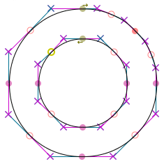
 Fig. 1 An outline of a degree symbol from DejaVu Sans font.
The previous article in the series explored drawing circles with linear Bézier curves. This article continues by showing how to use quadratic curves. Table of Contents
A quadratic Bézier curve uses three control points. The first and last points are the endpoints, while the middle one provides control over the curve’s shape. This additional control lets quadratic curves approximate curved shapes more accurately. Although they’re less expressive than higher-order curves, quadratic curves are widely used thanks to their balance of computational complexity and shape control — most notably in computer fonts (see Fig. 1) where the relative simplicity enables efficient rendering algorithms.1
A quadratic Bézier curve is constructed using the de Casteljau algorithm where adjacent control points act as endpoints for linear interpolation, creating a new sequence with one fewer point than the last. This process repeats until one point remains, yielding a point on the curve.2 Fig. 2 visualises the procedure for a quadratic Bézier curve.(JavaScript support is required to see the figure).
Fig. 2 De Casteljau construction of a quadratic Bézier curve. The point on the curve \( \def\tau2k{\frac τ{2k}} \def\O{\mathbf O} \def\P{\mathbf P} \def\Q{\mathbf Q} \def\argmin{\operatorname*{arg\,min}} \def\lerp{\operatorname{lerp}} B\) is linearly interpolated between points \(\Q_0\) and \(\Q_1\) which themselves are linearly interpolated between \(\P_0\) and \(\P_1\), and \(\P_1\) and \(\P_2\) respectively.
Based on the de Casteljau algorithm, a closed-form equation for the curve is derived as follows: $$\begin{align} \lerp(a, b, t) &= (1-t)a + tb \\[.5em] \Q_0(t) &= \lerp(\P_0, \P_1, t) = (1-t)\P_0 + t\P_1 \\ \Q_1(t) &= \lerp(\P_1, \P_2, t) = (1-t)\P_1 + t\P_2 \\ B(t) &= \lerp(\Q_0(t), \Q_1(t), t) \\ &= (1-t)\bigl((1-t)\P_0 + t\P_1\bigr) + t\bigl((1-t)\P_1 + t\P_2\bigr) \\ &= (1-t)^2\P_0 + 2(1-t)t\P_1 + t^2\P_2 \end{align}$$
Drawing a circle
To draw a circle, several Bézier curves are connected end-to-end forming a Bézier spline or a composite Bézier curve. For example, a spline consisting of two quadratic curves (or two segments) is described by a sequence of five points: \((\P_0, \P_1, \P_2, \P_3, \P_4)\). The first curve uses control points \((\P_0, \P_1, \P_2)\) and the second uses \((\P_2, \P_3, \P_4)\). The points that denote the start or end of a curve (\(\P_0, \P_2\) and \(\P_4\) in the example) are called anchors. Anchors shared between curves of the spline (\(\P_2\) in the example) are called joints. The remaining points are called handles. Fig. 3 demonstrates an example spline.Fig. 3 A two-segment quadratic Bézier spline.
To approximate a circle using \(k\) quadratic Bézier curves, \(2k+1\) control points are used. Even control points (joints) are spread equally on a circle of radius \(r\) (cf. vertices of a regular polygon), while odd control points (handles) are placed in-between on a circle of radius \(h\). Optimising the \(r\) and \(h\) parameters makes the spline resemble a circle more closely.
Choosing the parameters and smoothness
The previous article introduced the radial drift (or just drift) to estimate accuracy of a circle approximation. The same measure is used to optimise the parameters of a quadratic Bézier spline. However, accuracy is not the only consideration.
Fig. 4 presents a joint of a four-segment spline approximating a circle. The spline minimises the maximum absolute drift but, as a result, contains a sharp corner which is undesirable in applications such as animation. An object travelling along the shape abruptly changes direction at the joint, resulting in a jarring motion.Fig. 4 A sharp joint in an approximation of a circle built from four Bézier curves. Dashed line is the circle being approximated.
For smooth animation, an object’s velocity must change continuously, avoiding sudden jumps. Mathematically, this is the concept of continuity and specifically parametric continuity. A shape is \(C^0\) continuous if it has no gaps. By construction, all splines are \(C^0\) continuous. It’s \(C^1\) continuous if its first derivative is \(C^0\) continuous.3 In general, a \(C^m\) continuous path has continuous derivatives up to the order \(m\). A quadratic Bézier spline approximating a circle is at most \(C^1\) continuous (see appendix I).
A more permissive form of continuity is geometric continuity, denoted \(G^m\). \(G^0\) continuity requires the shape to have no gaps (i.e. \(G^0=C^0\)). A \(G^1\) continuous curve is one where tangent along the shape changes smoothly. Every \(C^m\)-continuous curve is also \(G^m\) continuous; parametric continuity is therefore a subset of geometric continuity: \(G^0=C^0⊃G^1⊃C^1⊃⋯⊃G^∞=C^∞\). Geometric continuity is important in achieving visual smoothness of a shape.4
In a Bézier spline, a line connecting a joint and neighbouring handle is tangent to the curve at the joint. For a Bézier spline (of any order) to be \(G^1\) continuous, a joint and its two surrounding handles must be collinear. For it to be \(C^1\) continuous, the handles must be equidistant from the joint.
The trade-off of requiring a smooth approximation is a constraint on the \(r/h\) ratio, which keeps the spline from reaching the lowest possible maximum absolute drift. This is shown in Fig. 5, an interactive demonstration comparing different splines.Fig. 5 Interactive demonstration of two different methods of drawing a circle with quadratic Bézier curves. Requires JavaScript to function.
To approximate a circle of radius \(R\) by \(k\) quadratic Bézier curves, the curves are joined to form a quadratic Bézier spline with the following \(2k+1\) control points from \(\P_0\) to \(P_{2k}\) where \(\P_0=\P_{2k}\). The approximation is parameterised on with \(r\) and \(h\) variables which determine how closely the shape resembles the circle and are chosen depending on the requirements of the application. A smooth, \(C^1\) continuous approximation is appropriate, for example, in animation. When smoothness is not required, a tighter, \(C^0\) continuous approximation might suffice. Formulæ for the parameters are:
| $$\P_i=\begin{cases} \left(Rr\cos\frac{iτ}{2k}, Rr\sin\frac{iτ}{2k}\right) &\quad\text{if } i = 2j\\ \left(Rh\cos\frac{iτ}{2k}, Rh\sin\frac{iτ}{2k}\right) &\quad\text{if } i = 2j+1 \end{cases}$$ |
| Smooth approximation |
|---|
| $$r = h\cos\tau2k\qquad h = \frac4{(\cos\tau2k+1)^2}$$ |
| Non-smooth approximation |
|---|
| $$r = \frac4{2 + \sqrt{4-(\cos\tau2k - 1)^2}}\qquad h = r(2 - \cos\tau2k)$$ |
$$\begin{align}\P_0&=R·(r, 0)\\ \P_1&=R·(a, a)\\ \P_2&=R·(0, r)\end{align}$$ The remaining points are generated using \(\mathbf ρ_{90°}(x,y)=(-y, x)\) rotation function and \(P_{i+2}=ρ_{90°}(\P_i)\) relation. |
| Smooth approximation |
|---|
| $$\begin{align}r &= 12\sqrt 2-16 ≈ 0.970562748477141\\ a &= r\end{align}$$ |
| Non-smooth approximation |
|---|
| $$\begin{alignat}{2}r &= \frac8{4 + \sqrt{10+4\sqrt 2}} &&≈ 1.00541992940814\\ a &= r\left(\sqrt 2 - 0.5\right) &&≈ 0.919168535345119\end{alignat}$$ |
$$\begin{split} &\P_0=R·(a, 0)\\ &\P_1=R·(b, c)\\ &\P_2=R·(d, d)\\ &\P_3=R·(c, b)\\ &\P_4=R·(0, a) \end{split}$$ The remaining points are generated using \(\mathbf ρ_{90°}(x,y)=(-y, x)\) rotation function and \(P_{i+2}=ρ_{90°}(\P_i)\) relation. |
| Smooth approximation |
|---|
| $$\begin{align} a&= \frac{8q}{(q+2)^2} ≈ 0.998434521365007\\ b&= a\\ c&= a\left(\sqrt 2 - 1\right)≈ 0.413565119890876\\ d&= \frac a{\sqrt 2} ≈ 0.705999820627941\\ &\text{where:}\\ q &= \sqrt{2+\sqrt 2} \end{align}$$ |
| Non-smooth approximation |
|---|
| $$\begin{align} a &= \frac8E ≈1.00036240788439\\ b &= F\sqrt{2+\sqrt 2}≈0.994565982404420\\ c &= F\sqrt{2-\sqrt 2}≈0.411962718586832\\ d &= \frac a{\sqrt 2} ≈0.707363042259156\\ &\text{where:}\\ q &= \sqrt{2+\sqrt 2}\\ E &= 4+\sqrt{16 - \left(2 - q\right)^2}\\ F &= \frac{8-2q}E \end{align}$$ |
Drift comparison
Fig. 6 compares the maximum absolute drift of \(C^0\) continuous and \(C^1\) continuous splines with respect to the number of segments in a spline.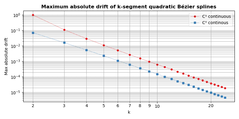 Fig. 6 Comparison of maximum absolute drift of quadratic Bézier splines with different number of segments and methods of picking their parameters. (Click to open the image).
Appendix
The appendix derives and justifies the formulæ presented in the article. §I derives the continuity constraints for quadratic Bézier splines, and §II applies them to a \(C^1\) continuous spline approximating a circle. The remaining sections find the \(r\) and \(h\) parameters for different approximation goals: §III sets up drift-minimisation problem and the notation used thereafter; §IV solves it for a \(C^1\) continuous spline; and §V solves it without continuity constraint.
I On continuity of Bézier splines
Bézier curves are polynomials and as such infinitely differentiable. A Bézier spline is \(C^1\) continuous if its first derivative at the joint points exists. Consider a two-segment quadratic Bézier spline defined by points \(\P_0\), \(\P_1\), \(\P_2\), \(\P_3\) and \(\P_4\). Let \(B_0\) and \(B_1\) represent the two segments of the spline, then: $$\begin{align} B_0(t) &= (1-t)^2\P_0 + 2(1-t)t\P_1 + t^2\P_2\\ B'_0(t) &= (2t-2)\P_0 + 2(1-2t)\P_1 + 2t\P_2\\ &= 2\bigl(-(1-t)\P_0 + (1-t)\P_1 - t\P_1 + t\P_2\bigr)\\ &= 2\bigl((1-t)(\P_1-\P_0) + t(\P_2-\P_1)\bigr)\\ &= 2\lerp(\P_1-\P_0, \P_2-\P_1, t)\\ B'_1(t) &= 2\lerp(\P_3-\P_2, \P_4-\P_3, t)\\ \end{align}$$
The derivative of a quadratic Bézier curve is a scaled linear Bézier curve with differences between adjacent points as control points (the following article explores this further). To find the condition for \(C^1\) continuity we equate the first derivatives at the joint: $$\begin{align} B'_1(0) &= B'_0(1)\\ 2(\P_3-\P_2) &= 2(\P_2-\P_1)\\ \P_3 &= 2\P_2-\P_1\\ &= \P_2 - (\P_1-\P_2) \end{align}$$
Geometric interpretation is that a joint and its two surrounding handle points must be collinear and the handles must be equidistant from the joint. This condition generalises to Bézier splines of higher order.
Next, we ask what condition is necessary for the spline to be \(C^2\) continuous. This requires looking at the second derivatives at the joint: $$\begin{align} B''_0(t) &= 2\bigl(-(\P_1-\P_0)+(\P_2-\P_1)\bigr)\\ &= 2(\P_0-2\P_1+\P_2)\\ B''_1(t) &= 2(\P_2-2\P_3+\P_4)\\[.5em] B''_1(0) &= B''_0(1)\\ \P_2-2\P_3+\P_4 &= \P_0-2\P_1+\P_2\\ \P_4 &= \P_0-2\P_1+2\P_3\\ &= \P_0-2\P_1+2(2\P_2-\P_1)\\ &= \P_0-4\P_1+4\P_2\\ &= \P_0-4(\P_1-\P_2) \end{align}$$
Pursuing \(C^2\) continuity means the control points of the second segment are determined by the control points of the first one. In fact, a \(C^2\) quadratic Bézier spline is fully defined by the equation of its first segment. The spline is a continuation of the curve created by taking the parameter \(t\) outside the \([0, 1]\) range, as is shown below: $$\begin{align} B_0(1+x) &= (1-1-x)^2\P_0 + 2(1-1-x)(1+x)\P_1 + (1+x)^2\P_2\\ &= x^2\P_0 - 2x(1+x)\P_1 + (1+x)^2\P_2\\ &= x^2\P_0 - 2(x + x^2)\P_1 + (1 + 2x + x^2)\P_2\\ &= x^2\P_0 + (-2x + 2x^2 - 4x^2)\P_1 + (1 - 2x + x^2 + 4x - 4x^2 + 4x^2)\P_2\\ &= (1-x)^2\P_2 + 2(x-x^2)(2\P_2-\P_1) + x^2(\P_0-4\P_1+4\P_2)\\ &= (1-x)^2\P_2 + 2(1-x)x\P_3 + x^2\P_4\\ &= B_1(x) \end{align}$$
This generalises to higher order splines: requiring a Bézier spline of order \(n\) to have \(C^m\) continuity ‘locks’ the first \(m\) handles of all but the first curve in the spline. If \(m≥n\), the entire spline is fully defined by the first curve.
II Creating smooth approximation
By §I, a Bézier spline is \(C^1\) continuous if and only if each joint and the two control points surrounding it are collinear. Due to symmetry of a circle approximation, this translates to the handles being at intersection of the tangents as shown in Fig. 8.$$ |∢\P_0\O\P_1| = |∢\P_2\O\P_1| = φ\\ |∢\O\P_0\P_1| = |∢\O\P_2\P_1 = \frac τ4\\ \cosφ = \frac rh $$
Let \(r_s\) and \(h_s\) denote the parameters of a smooth approximation. The geometric constructions shows that \(r_s=h_s\cos\tau2k\) where \(k\) is the number of segments in the spline. This leaves one free variable which we look at next.
III Defining the drift minimisation problem
This section demonstrates how to obtain optimal parameters for a \(k\)-segment quadratic Bézier spline approximating a unit circle. By the rotational symmetry of the spline, without loss of generality, we look at a single curve whose control points are symmetric about the horizontal axis. For brevity, let \(C=\cos\tau2k\) and \(S=\sin\tau2k\). $$\begin{align} \P_0 &= (rC, \phantom-rS)\\ \P_1 &= (h, 0)\\ \P_2 &= (rC, -rS) \end{align}$$
To take advantage of the symmetry, rather then expressing the curve as a function of parameter \(0≤t≤1\), use \(u=t-0.5\) substitution. Furthermore, let \(p=0.5-u\) and \(q=0.5+u\): $$\begin{align} X_{r,h}(u) &= p^2rC + 2pqh + q^2rC\\ &= (p^2+q^2)rC + 2pqh\\ &= ((p+q)^2 - 2pq)rC + 2pqh\\ &= (1 - 2(0.25 - u^2))rC + 2(0.25 - u^2)h\\ &= (2u^2 + 0.5)rC - (2u^2 - 0.5)h\\[.5em] Y_{r,h}(u) &= p^2rS + 2pq·(0) - q^2rS\\ &= (p^2-q^2)rS = (p-q)rS\\ &= -2urS\\ B_{r,h}(t) &= \bigl(X_{r,h}(t-0.5), Y_{r,h}(t-0.5)\bigr) \end{align}$$
Let \(D\) denote distance of the point on the curve from the origin. $$\begin{align} D_{r,h}(u) &= |B_{r,h}(u+0.5)|\\ &= \sqrt{X_{r,h}(u)^2 + Y_{r,h}(u)^2}\\ X_{r,h}(u)^2 &= (2u^2 + 0.5)^2r^2C^2\\ &{}- 2(2u^2 + 0.5)(2u^2 - 0.5)rCh\\ &{}+ (0.5 - 2u^2)^2h^2\\ &= (4u^4 + 2u^2 + 0.25)r^2C^2\\ &{}- 2(4u^4 - 0.25)rCh\\ &{}+ (4u^4 - 2u^2 + 0.25)h^2\\ Y_{r,h}(u)^2 &= 4u^2r^2S^2\\ D_{r,h}(u)^2 &= 4(r^2C^2 - 2rCh + h^2)u^4\\ &{}+ 2(2r^2S^2 + r^2C^2 - h^2)u^2\\ &{}+ \frac14(r^2C^2+2rCh+h^2)\\ &= 4(rC-h)^2u^4\\ &{}+ 2(r^2(1+S^2)-h^2)u^2\\ &{}+ \frac14(rC+h)^2 \end{align}$$
Since \(D_{r,h}(u)^2\) is an even polynomial, \(v=u^2\) substitution reduces its degree. Let \(a, b, c\) and \(d_{r,h}(v)\) be defined as follows: $$\begin{align} a &= 4(rC-h)^2\\ b &= 2(r^2(1+S^2)-h^2)\\ c &= \frac14(rC+h)^2\\ d_{r,h}(v) &= av^2+bv+c\\ \end{align}$$
By construction, \(D_{r,h}(0.5) = \sqrt{d_{r,h}(0.25)} = r\) (because endpoints of the Bézier curve are \(r\) units away from origin). Minimising the maximum absolute drift, we look for \(r^*,h^*\) pair such that: $$\begin{align} (r^*, h^*) &= \argmin_{r,h>0} \max_{0≤t≤1} \bigl||B_{r,h}(t)|-1\bigl|\\ &= \argmin_{r,h>0} \max_{-0.5≤u≤0.5} |D_{r,h}(u)-1|\\ &= \argmin_{r,h>0} \max_{0≤v≤0.25} \left|\sqrt{d_{r,h}(v)}-1\right| \end{align}$$
To find the maximum, points from three categories need to be checked.5
- The endpoints of the interval: 0 and 0.25.
- The critical points of \(d_{r,h}\). Since it’s a parabola, its derivative reaches zero at the vertex \(v^* = -b/(2a)\). So long as the point is within \((0, 0.25)\) range, it needs to be checked.
- The points where \(d_{r,h}(v)=1\). However, \(|\sqrt{d_{r,h}(v)}-1|\) cannot attain a unique maximum at those points, so they may be ignored.
With those definitions, we move to optimising the shape of quadratic splines approximating the unit circle.
IV Optimising the smooth approximation
Applying the \(r_s=hC\) constraint removes one free variable from the smooth approximation defined in §II and simplifies the problem to: $$h_s = \argmin_{h>0} \max_{0≤v≤0.25} \left|\sqrt{d_{r_s,h}(v)}-1\right|$$
First, compute the coefficients of \(d_{r_s,h}\); let’s call them \(a_s\), \(b_s\) and \(c_s\): $$\begin{align} a_s &= 4(r_sC-h)^2\\ &= 4(hC^2-h)^2\\ &= 4h^2S^4\\ b_s &= 2(r_s^2(1+S^2)-h^2)\\ &= 2(h^2C^2(1+S^2)-h^2)\\ &= 2h^2(C^2 - 1 + C^2S^2)\\ &= 2h^2(C^2S^2 - S^2)\\ &= 2h^2S^2(C^2 - 1)\\ &= -2h^2S^4\\ c_s &= \frac14(r_sC+h)^2\\ &= \frac14(hC^2+h)^2\\ &= \frac{h^2}4(C^2+1)^2 \end{align}$$
Observe that \(a_s = -2b_s\). The vertex of the \(d_{r_s,h}\) parabola is \(-b_s/(2a_s) = -b_s/(2(-2b_s)) = 0.25\) which falls at the boundary of \([0, 0.25]\) interval. Substituting these coefficients into the \(d_{r_s,h}\) yields: $$\begin{align} d_{r_s,h}(v) &= a_sv^2 + b_sv + c_s\\ &= -2b_sv^2 + b_sv + c_s\\ &= b_s(-2v+1)v + c_s\\ &= -2h^2S^4(-2v+1)v + \frac{h^2}4(C^2+1)^2\\ &= h^2\left(2S^4(2v-1)v + \frac14(C^2+1)^2\right) \end{align}$$
Let \(Ç=(C^2+1)/2\) and so: $$\begin{align} h_s &= \argmin_{h>0} \max \left\{\left|\sqrt{d_{r_s,h}(0)}-1\right|, \left|\sqrt{d_{r_s,h}(0.25)}-1\right|\right\}\\ &= \argmin_{h>0} \max \left\{\left|\sqrt{h^2Ç^2}-1\right|, |r_s-1|\right\}\\ &= \argmin_{h>0} \max \bigl\{|hÇ-1|, |hC-1|\bigr\} \end{align}$$
Because \(hÇ-1\) and \(hC-1\) are straight lines with positive slope and distinct zeros, the minimum argument is found if branches of the max operator are balanced,5 i.e.: \(h_sÇ-1=1-h_sC\) which yields \(h_s(Ç+C)=2 ⇔ h_s = 2/(Ç+C)\) and so: $$\begin{align} Ç+C&=\frac{C^2+1}2+C=\frac{(C+1)^2}2\\ h_s&=\frac2{Ç+C}=\frac{4}{(C+1)^2} \end{align}$$
Finally, the closed-form formulæ for the optimal \(r_s\) and \(h_s\) parameters of a \(C^1\) continuous \(k\)-segment Bézier spline approximating a unit circle:
$$h_s=\frac4{(\cos\tau2k+1)^2}\\r_s=h_s\cos\tau2k$$
The maximum absolute drift for such an approximation is: $$\begin{align} 1-h_sC&=1-\frac{4C}{(C+1)^2}\\ &=\frac{C^2+2C+1-4C}{(C+1)^2}\\ &=\frac{(C-1)^2}{(C+1)^2}\\ \end{align}$$
$$\max\bigl||B_{r_s,h_s}(t)|-1\bigr|= \frac{(\cos\tau2k-1)^2}{(\cos\tau2k+1)^2}$$
V Optimisation without smoothness constraint
If the \(C^1\) continuity of the shape is not a concern, a quadratic Bézier spline can be optimised further. Because the optimisation problem defined in §III has no clean closed-form solution, this section uses a hybrid approach: closed-form formulæ combined with numerical validation.
First, assume equioscillation, i.e. that the drift oscillates at its active points between \(-δ\) and \(δ\) where \(δ\) is the maximum absolute drift. This provides sufficient constraints to find closed-form formulæ for the parameters. The method works when fitting polynomials, but is not guaranteed to give optimal results in our case where the \(d\) function isn’t convex.7. Second, because the equioscillation assumption isn’t guaranteed to be optimal, numeric methods validate the solution empirically. While not a mathematical proof, this approach is enough for practical application.
Assuming equioscillation
From §III, \(d\) is a parabola over \(v\) and the three active points when evaluating the maximum are: 0, vertex of the parabola \(v^*\) and 0.25. Let \(r_e\) and \(h_e\) be the parameters at which equioscillation occurs, then: \(\sqrt{d_{r_e,h_e}(0)}-1 = 1-\sqrt{d_{r_e,h_e}(v^*)} = \sqrt{d_{r_e,h_e}(0.25)}-1\). First, look at the constraint introduced by the points at the 0 and 0.25: $$\begin{align} \sqrt{d_{r_e,h_e}(0.25)} - 1 &= \sqrt{d_{r_e,h_e}(0)} - 1\\ r-1 &= \frac{rC + h}2\\ 2r &= rC + h\\ h_e &= r(2 - C) = 2r - rC\\ \end{align}$$
This result simplifies coefficients of \(d_{r,h_e}\); let’s call them \(a_e\), \(b_e\) and \(c_e\): $$\begin{align} a_e&= 4(rC-h_e)^2\\ &= 4(rC-2r+rC)^2\\ &= 16r^2(C-1)^2\\ b_e&= 2(r^2(1+S^2)-h_e^2)\\ &= 2(r^2(2-C^2)-r^2(2 - C)^2)\\ &= 2r^2(2-C^2-(4 - 4C + C^2))\\ &= 2r^2(-2+4C-2C^2)\\ &= -4r^2(C - 1)^2\\ c_e&= \frac14(rC+h_e)^2\\ &= \frac14(rC+2r-rC)^2\\ &= r^2 \end{align}$$
With that, equate the drift at the boundary to negative of the drift at the vertex. For this to be valid, first check that the vertex falls in \((0, 0.25\)) interval. Observe that \(a_e = -4b_e\) from which it follows that the position of the vertex is \(-b_e/(2a_e) = -b_e/(2(-4b_e)) = 1/8\).
By the properties of a parabola, value at vertex is \(d_e^* = c_e - b_e^2/(4a_e) = c_e - b_e^2/(4(-4b_e)) = c_e + b_e/16\) which results in: $$\begin{align} \sqrt{d_{r_e,h_e}(0.25)}-1 &= 1 - \sqrt{d{r_e,h_e}(v^*)}\\ r - 2 &= -\sqrt{d_e^*}\\ r^2 - 4r + 4 &= c_e + \frac{b_e}{16}\\ r^2 - 4r + 4 &= r^2 + \frac{-4r^2(C - 1)^2}{16}\\ 4r - 4 &= r^2\frac{(C - 1)^2}4\\ 16r - 16 &= r^2(C - 1)^2 0 &= r^2(C - 1)^2 - 16r + 16 \end{align}$$
For brevity, let \(Ć=(C-1)^2\) and so: $$\begin{align} Δ &= (-16)^2 - 4Ć(16)\\ &= 64(4 - Ć)\\ r &= \frac{-(-16) ± \sqrt{Δ}}{2Ć}\\ &= \frac{16 ± 8\sqrt{4 - Ć}}{2Ć}\\ &= 4\frac{2 ± \sqrt{4 - Ć}}{Ć}\\ &= 4\frac{(2 ± \sqrt{4-Ć})(2 ∓ \sqrt{4-Ć})}{Ć(2 ∓ \sqrt{4-Ć})}\\ &= 4\frac{4-4+Ć}{Ć(2 ± \sqrt{4-Ć})}\\ &= \frac4{2 ± \sqrt{4-Ć}}\\ \end{align}$$
The minus branch yields value far from optimal and can be discarded. This leaves a unique solution for parameters of a \(k\)-segment Bézier spline:
$$r_e = \frac4{2 + \sqrt{4-(\cos\tau2k-1)^2}}\\ h_e = r_e(2 - \cos\tau2k)$$
Evaluating the drift at the anchor gives the maximum absolute drift: $$\begin{align} r_e-1 &= \frac4{2 + \sqrt{4-Ć}} - 1\\ &= \frac{4 - 2 - \sqrt{4-Ć}}{2 + \sqrt{4-Ć}}\\ &= \frac{2 - \sqrt{4-Ć}}{2 + \sqrt{4-Ć}} \end{align}$$
$$ max\bigl||B_{r_e,h_e}(t)|-1\bigr|=\frac{2-F}{2+F}\\ \text{where } F = \sqrt{4-\left(\cos\tau2k-1\right)^2} $$
Validating the result
Although we’ve identified some parameters which provide favourable results, we haven’t shown a superior pair doesn’t exist. To justify that the result is optimal, we use numerical methods to search for a better parameters.
We employ SciPy for that purpose. It is a Python library which, among other things, implements various optimisation algorithms. Its scipy.optimize.minimize function takes an objective function, initial guess and parameter bounds to find the parameters which minimise the objective. Invocation of the function is as follows:
import scipy

def max_abs_drift(k: int, r: float, h: float) -> float:
        ...

def minimise(
                k: int,
                initial_guess: tuple[float, float],
                method: str,
) -> scipy.optimize.OptimizeResult:
        objective = lambda params: abs(
                max_abs_drift(k, *params))
        return scipy.optimize.minimize(
                objective,
                initial_guess,
                bounds=((0.5, 1.5), (0.5, 2.5)),
                method=method)
The minimise function uses given method (i.e. optimisation algorithm) to find optimal spline parameters. It needs to determine maximum absolute drift for a spline with particular parameters. This calculation is handled by the max_abs_drift function.
The function evaluates \(\max_{0≤t≤1} \bigl||B_{r,h}(t)|-1\bigl|\) from §III. First, it identifies active points of the \(\max\) expression in terms of \(v\) and then undoes the \(t→u→v\) substitution to recover corresponding \(t\) values. By §III, relevant values are \(v∈\{0, v^*, 0.25\}\) which maps to \(t∈\{0, t_-^*, 0.5, t_+^*, 1\}\) points where: $$\begin{align} v^*&= \frac{-b}{2a}\\ &= \frac{-2(r^2(1+S^2)-h^2)}{2·4(rC-h)^2}\\ &= \frac{h^2-r^2(2-C^2)}{4(rC-h)^2}\\ t^*&= 0.5±\sqrt{v^*}\\ &= 0.5±\frac{\sqrt{h^2+r^2(C^2-2)}}{2|rC-h|} \end{align}$$
By the symmetry of \(B_{r,h}\) about 0.5, values (\t>1/2\) can be ignored and only the minus branch is relevant. Putting this together, max_abs_drift becomes:
import math

Point = tuple[float, float]

def bezier(points: tuple[Point, ...],
           t: float) -> Point:
        ...

def max_abs_drift(k: int, r: float, h: float) -> float:
        phi = math.pi / k
        c, s = math.cos(phi), math.sin(phi)
        points = ((r*c, r*s), (h, 0), (r*c, -r*s))

        active_points: tuple[float, ...] = (0, 0.5)
        radicand = h*h + r*r*(c*c - 2)
        denom = r*c - h
        if denom != 0 and radicand > 0:
                root = math.sqrt(radicand)
                t = 0.5 - root / abs(2*denom)
                if t > 0:
                        active_points = (0, t, 0.5)

        values = (abs(math.hypot(*bezier(points, t)) - 1)
                  for t in active_points)
        return max(values)
For the bezier implementation, use the de Casteljau algorithm which has a concise implementation in Python:
def lerp(a: Point, b: Point, t: float) -> Point:
        return ((1-t)*a[0] + t*b[0],
                (1-t)*a[1] + t*b[1])

def bezier(points: tuple[Point, ...],
           t: float) -> Point:
        while len(points) > 1:
                pairs = zip(points, points[1:])
                points = tuple(lerp(a, b, t)
                               for a, b in pairs)
        return points[0]
The minimise function is used to compare the analytically derived parameters to those found numerically. If numerical methods fail to find an improvement, we can be reasonably sure that the closed-form formulæ are correct. To give the numeric approach the best chance, it uses multiple algorithms and initial guesses:
def smooth_params(k: int) -> tuple[float, float]:
        ...

def best_params(k: int) -> tuple[float, float]:
        ...

methods = ('Nelder-Mead', 'L-BFGS-B', 'TNC', 'SLSQP')
ok = True
for k in range(3, 100):
        smooth = smooth_params(k)
        params = best_params(k)
        guesses = ((1.0, 1.0), smooth, params)
        result = min((minimise(k, guess, method)
                      for guess in guesses
                      for method in methods),
                     key=lambda result: result.fun)
        drift = max_abs_drift(k, *params)
        if drift <= result.fun:
                continue

        rel_diff = (drift - result.fun) / result.fun
        if rel_diff < 1e-6:
                msg = ', close enough'
        else:
                msg = ''
                ok = False
        print(f'k = {k:3}: {drift} > {result.fun}'
              f' ({rel_diff * 100:.3}% worse){msg}')

if not ok:
        raise SystemError('Better parameters found')
smooth_params and best_params return spline parameters as derived in §II and Assuming equioscillation subsection respectively. The functions consist of straightforward calculations:
def smooth_params(k: int) -> tuple[float, float]:
        cos = math.cos(math.pi / k)
        h = 4 / (1 + cos)**2
        r = h * cos
        return (r, h)

def best_params(k: int) -> tuple[float, float]:
        cos = math.cos(math.pi / k)
        r = 4 / (2 + math.sqrt(4 - (cos - 1)**2))
        h = r * (2 - cos)
        return (r, h)
Running the script shows that the formulæ are optimal — within a negligible numerical error — for \(k∈[3,99]\). The script finds six instances where numerical methods produced an improvement listed in the table below. Each improvement was by than one part in a million and is likely a result of floating point calculation inaccuracies.
| k | Maximum absolute drift | Relative change |
|---|
| Analytical solution | Numerical solution |
|---|
| 3 | 0.01613323034066516 | 0.01613323034066505 | 6.88e-13% |
| 20 | 9.47373933235518e-06 | 9.473739332244158e-06 | 1.17e-09% |
| 46 | 3.3966504875415637e-07 | 3.3966504864313407e-07 | 3.27e-08% |
| 60 | 1.1738596461530193e-07 | 1.1738596450427963e-07 | 9.46e-08% |
| 65 | 8.523090033740743e-08 | 8.523090022638513e-08 | 1.3e-07% |
| 76 | 4.560805022535419e-08 | 4.560805011433189e-08 | 2.43e-07% |
Full code to perform the validation (though not exactly the code presented here) with functions for Bézier interpolation and optimisation can be found in the bezier-circles repository.1 Scuff3D Rook. 2026. The Scanline Sweeper: A Glyph Rendering Algorithm. Rook & Possum. https://rookandpossum.com/posts/scanline-sweeper/. ↩
2 Wolfgang Boehm, Andreas Müller. 1999. On de Casteljau’s algorithm. Computer Aided Geometric Design, Vol. 16, Issue 7 (Aug. 1999). 587–605. doi:10.1016/S0167-8396(99)00023-0. ↩
3 Thomas W. Sederberg. 2012. §2.10 Continuity. Computer Aided Geometric Design. http://hdl.lib.byu.edu/1877/2822. ↩
4 Freya Holmér. 2022. The Continuity of Splines. Video. https://youtu.be/jvPPXbo87ds. ↩
5 Donald A. Pierre. 1986. §2-3. Functions of one variable. Optimization theory with applications. Dover Publications, New York, NY, USA. 31–35. ISBN 0-486-65205-X. ↩
6 Stephen Boyd, Lieven Vandenberghe. 2004. Convex Optimization. Cambridge University Press, Cambridge, UK. ISBN 978-0-521-83378-3. https://web.stanford.edu/~boyd/cvxbook/. ↩
7 Lloyd N. Trefethen. 2019. Approximation Theory and Approximation Practice, Extended Edition. Society for Industrial and Applied Mathematics, Philadelphia, PA, USA. doi:10.1137/1.9781611975949. ISBN 978-1-61197-593-2. ↩