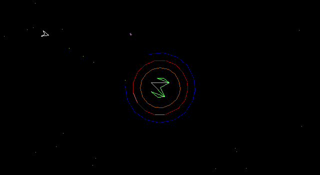
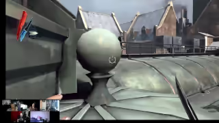
 Fig. 1 First: Star Castle video game draws circles as regular polygons. Second: Dishonored draws a round finial with straight edges (screenshot thanks to Raphael Colantonio). (Click to open the image).
Some systems do not provide a circle primitive; in those cases, circles need to be approximated using different shapes. For example, many fonts are limited to quadratic Bézier curves,1 and even though Adobe Animate includes a circle tool, it represents circles using cubic Bézier curves instead.2 Such approximations are common in video games as well (see Fig. 1), where round objects still present rendering challenges.
This post is first in a series of articles about approximating circles. It introduces linear Bézier curves, and how to approximate a circle using linear Bézier curves. The next two articles cover quadratic and cubic curves, which produce progressively smoother results. Table of Contents
Linear Bézier curves
Originally developed for automotive design, Bézier curves are often used in computer graphics, computer-aided design (CAD), simulation and other fields3. They are supported by SVG paths, offered in CSS as an interpolating function, used to define outlines in font files and available in virtually any graphics editor. A Bézier curve is defined by a sequence of control points \( \def\tau2k{\frac τ{2k}} \def\P{\mathbf P} \def\argmin{\operatorname*{arg\,min}} \def\sgn{\operatorname{sgn}} \P_0, \P_1, …, \P_n\) where \(n≥1\) is the degree of the curve. Although Bézier curves of degrees two and three are common, it’s useful to begin with the simplest possible case: a linear Bézier curve.
A linear Bézier curve has two control points and is simply another way of describing a straight line. It has a parametric formula equivalent to linear interpolation (or lerp): \(B(t) = (1-t)\P_0 + t\P_1\). As a result, approximating a circle with linear Bézier curves reduces to constructing a regular \(k\)-gon whose vertices are: \(\P_i = \left(r\cos(iτ/k), r\sin(iτ/k)\right)\) for \(i = 0, 1, …, k-1\).
Choosing the size of the polygon
For a given \(k\)-gon, this leaves one free parameter: \(r\). One might initially expect it to equal the radius of the circle being approximated, but the situation is more complex. The main approaches, each with its own advantages depending on the application, are: inscribing the polygon, circumscribing the polygon and minimising the circle’s distortion.
Inscribing the polygon produces a shape contained within the circle; circumscribing it yields a shape completely enclosing the circle. However, both approaches concentrate distortion either at the vertices of the polygon or in the middle of its sides.
Radial drift, or just drift, puts a number to the distortion; it measures the distance between a point on the polygon and the circle. Since we’re using a regular polygon, it’s sufficient to consider just one of its sides. This yields the following formula for drift: \((|B(t)| - R)/R\) (where \(R\) is radius of the circle). Fig. 2 visualises it using a pentagon as an example.Fig. 2 Visualisation of drift for a pentagon approximating a circle. The thick red lines highlight drift measured along selected radii of the circle. The shaded area shows overall drift.
There are a few ways to minimise drift. A common approach, adapted from statistics, is to minimise the mean squared error (MSE), treating drift as the error term. It considers distortion along the entire polygon edge. While looking at MSE is a reasonable choice, an even better approach is to minimise the maximum absolute drift directly. It prioritises reducing the worst-case deviations while allowing the error to be spread over the edge. Fig. 3 demonstrates drift for four different polygons optimised based on these criteria.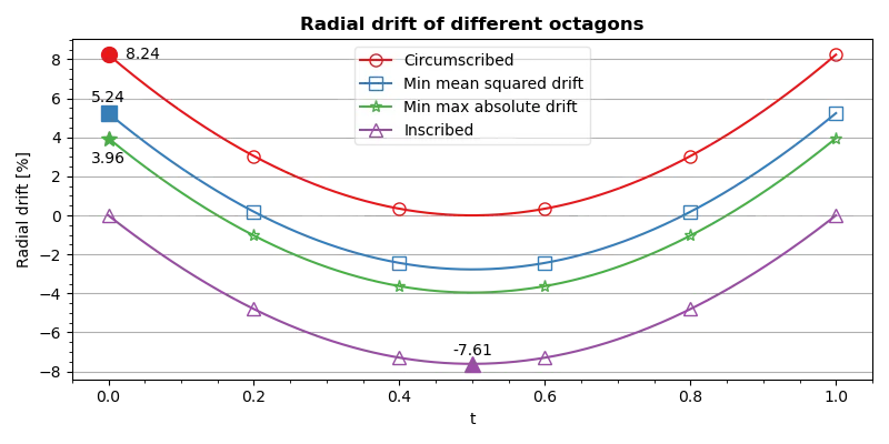 Fig. 3 Graph comparing the drift of different methods of specifying the size of the octagon. Labelled points mark maximum absolute drift for each method. (Click to open the image).
A circle of radius \(R\) is approximated by a regular \(k\)-gon whose vertices are: $$\P_i = \left(Rr\cos\frac{iτ}k, Rr\sin\frac{iτ}k\right)$$
for \(i = 0, 1, …, k-1\) where the \(r\) parameter determines the size of the polygon (in proportion to the size of the circle). It is chosen based on the requirements of the approximation. Minimising maximum absolute drift provides a polygon whose sides are closest to the circle, but in some applications inscribing or circumscribing the polygon may be preferred. The table below lists formulæ for the \(r\) parameter in order of increasing resulting maximum absolute drift:| Method | \(r\) | Max absolute drift |
|---|
| Minimise maximum absolute drift | $$\frac2{1+\cos\tau2k}$$ | $$\tan^2{\frac τ{4k}}$$ |
|---|
| Minimise mean squared drift | See \(r_m\) below. | See \(d_m\) below. |
|---|
| Inscribe | $$1$$ | $$1 - \cos\tau2k$$ |
|---|
| Circumscribe | $$\sec\tau2k$$ | $$\sec\tau2k-1$$ |
|---|
$$\begin{align} r_m &= \frac{3(2+A)}{4(1+2\cos^2ψ)}\\ d_m &= max \left\{|r_m-1|, |r_m\cos\tau2k - 1|\right\}\\ &\hspace{-1em}\text{where: }\\ A &= \frac{\cos^2ψ}{\sinψ} \ln\left(\frac{1+\sinψ}{1-\sinψ}\right)\\ ψ &= \tau2k \end{align}$$
For derivation of the formulæ, see appendix. For an interactive illustration, Fig. 4 lets you compare effects of different polygon sizing methods.Fig. 4 Interactive demonstration of four different methods of drawing a circle as a regular polygon. Requires JavaScript to function.
Fig. 5 plots the maximum absolute drift against the number of sides of the polygon and compares the drift attained by circumscribed polygons, inscribed polygons and polygons that minimise maximum absolute drift. Minimising mean squared drift produces maximum absolute drift only marginally worse than that attained by minimising the maximum absolute drift.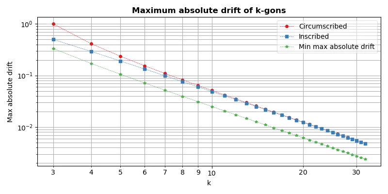 Fig. 5 Graph comparing the maximum absolute drift of polygons with different number of sides and methods of scaling their size. (Click to open the image).
The maximum absolute drift of inscribed and circumscribed polygons is roughly twice as large as that of optimally scaled polygons. Intuitively, this is because inscribed and circumscribed polygons have drift that never changes sign, while optimising the drift balances positive and negative drift.
Appendix
The appendix derives the formulæ for polygons that I) circumscribe a unit circle, II) minimise maximum absolute drift and III) minimise mean squared drift. In the equations \(k≥3\) denotes the number of sides of the polygon and \(r>0\) denotes the radius of the polygon, i.e. the distance of its vertices from its geometric centre.
For brevity, let \(C = \cos(τ/(2k))\) and \(S = \sin(τ/(2k))\). From \(k≥3\) it follows that \(0 < C, S < 1\). Without loss of generality, we assume the two endpoints of the line are placed symmetrically about the vertical axis, with one endpoint in the first quadrant: \(\P_0 = (rC, rS)\), and the other in the fourth: \(\P_1 = (rC, -rS)\). With those control points: $$\begin{align} B_r(t) &= (1-t) \P_0 + t \P_1\\ &= \bigl( rC, (1-t) rS - trS \bigr)\\ &= \bigl( rC, (1-2t) rS \bigr) \end{align}$$
The function is symmetric around 0.5. To take advantage of it, we use \(t=u+0.5\) substitution and define a new function measuring distance of a point from the origin: $$\begin{align} D_r(u) &= |B_r(u+0.5)|\\ &= |(rC, -2urS)|\\ &= r\sqrt{C^2 + 4u^2S^2}\\[.5em] \end{align}$$
Note that \(D_r(0)=rC\) and \(D_r(-0.5)=D_r(0.5)=r\).
I Circumscribed polygon
For a regular polygon to be circumscribed about a unit circle, its sides must touch the circle in the middle, that is \(1 = D_r(0) = rC\). Let \(r_c\) denote the radius of such a polygon, then:
$$r_c = \frac1{\cos\tau2k} = \sec\tau2k$$
To demonstrate the polygon doesn’t intersect the circle at any other points, we show \(D_r\) is strictly decreasing for \(u≤0\) and strictly increasing for \(u≥0\). To do so, we inspect the sign of its derivative: $$\begin{align} \sgn\frac{∂D_r}{∂u} &= \sgn\frac ∂{∂u} \left(r\sqrt{C^2 + 4u^2S^2}\right)\\ &= \sgn\frac ∂{∂u} (C^2 + 4u^2S^2)\\ &= \sgn 4uS^2\\ &= \sgn u \end{align}$$
Therefore \(D_r(u)>D_r(0)\) for \(u≠0\).
It’s also worth noting that the maximum absolute drift of an inscribed polygon is smaller than that of a circumscribed polygon: \(|D_1(0)-1| = |1C-1| = 1-C < (1-C)/C = 1/(C-1) = |D_{r_c}(-0.5)-1|\).
II Minimising maximum absolute drift
To find the polygon that best approximates a circle, we look for the parameter that minimises the absolute value of the drift: \(r_a = \argmin_{r>0} \max_{-0.5≤u≤0.5} |D_r(u)-1|\). To find the maximum, we check the following.4
- The endpoints of the interval: -0.5 and 0.5. Since \(D_r(-0.5)=D_r(0.5)\), it suffices to check \(0.5\).
- The critical points of \(D_r\). By §I, there is only one at zero.
- The points where \(D_r(u)=1\). However, \(|D_r(u)-1|\) attains its maximum at those points only if \(D_r≡1\), but in that case, checking those points is redundant, and so they may be ignored.
It follows that we only need to check values at 0 and 0.5: $$\begin{align} r_a &= \argmin_{r>0} \max \bigl\{|D_r(0)-1|, |D_r(0.5)-1|\bigr\}\\ &= \argmin_{r>0} \max \{|rC-1|, |r-1|\}\\ \end{align}$$
The absolute values of the linear expressions \(rC−1\) and \(r−1\) form two V-shaped graphs. Each decreases to zero and then increases, with opposite monotonicities between their roots. The minimum argument is found once the branches of the maximum are balanced:5 \(r_aC - 1 = -(r_a - 1) ⇔ r_aC + r_a = 2\). Therefore, to minimise the maximum absolute drift, the radius of the polygon must be:
$$r_a = \frac2{1 + \cos\tau2k} = \sec^2\frac τ{4k}$$
With that polygon’s radius, the maximum drift is \(D_{r_a}(0.5)-1 = 2/(1 + C) - 1 = (1 - C)/(1 + C\) or:
$$\max\bigl||B_{r_a}(t)|-1\bigr|= \frac{1 - \cos\tau2k}{1 + \cos\tau2k} = \tan^2\frac τ{4k}$$
III Minimising mean squared drift
Another way to optimise the accuracy of an approximation is to look at the mean squared drift. Let \(r_m\) be the radius of a polygon that minimises the mean squared drift, then: $$\begin{align} r_m&=\argmin_{r>0} \frac{∫_0^1 \bigl(|B_r(t)| - 1\bigr)^2 dt}{∫_0^1dt}\\ &=\argmin_{r>0} ∫_{-0.5}^{0.5} \bigl(D_r(u) - 1\bigr)^2 du \end{align}$$
Start by separating the parts of the integral that don’t depend on \(r\): $$\begin{align} I(r) &= ∫_{-0.5}^{0.5} \bigl(D_r(u) - 1 \bigr)^2 du\\ &= ∫_{-0.5}^{0.5} \left(r\sqrt{C^2 + 4u^2S^2} - 1\right)^2 du\\ &= \frac12∫_{-1}^1 \left(r\sqrt{C^2 + v^2S^2} - 1\right)^2 dv\\ &= \frac{r^2}2 ∫_{-1}^1 C^2 + v^2S^2\ dv\\ &{}- r ∫_{-1}^1 \sqrt{C^2 + v^2S^2}\ dv\\ &{}+ 1 \end{align}$$
Let \(I_1\) and \(I_2\) be the two sub-integrals such that \(I(r) = r^2I_1/2 - rI_2 + 1\). We want the \(r>0\) that minimises this integral. To find it, we identify critical points of \(I\) which requires differentiating it with respect to \(r\): $$\frac{dI}{dr} = \frac d{dr}\left(\frac{r^2}2 I_1 - rI_2 + 1\right) = rI_1 - I_2$$
The derivative has a single zero, where it flips from negative to positive. It follows that the minimum of the integral is reached at the critical point, i.e. \(r_m=I_2/I_1\). To find the final formula, we calculate the two sub-integrals. The first one is easily solved using the power rule: $$\begin{align} I_1 &= ∫_{-1}^1 C^2 + v^2S^2 \ dv\\ &= 2C^2 + \frac23S^2 = 2\frac{1+2C^2}3\\ \end{align}$$
The second integral takes the standard form \(∫\sqrt{ax^2 + c}\ dx\).5 For brevity, let \(Q(v) = \sqrt{v^2S^2 + C^2}\): $$\begin{align} I_2 &= ∫_{-1}^1 Q(v) dv\\ &= \left[ \frac v2Q(v) + \frac{C^2}{2S}\ln\bigl(Sv + Q(v)\bigr)\right]_{-1}^1\\ &= \frac12 + \frac{C^2}{2S}\ln(1 + S)\\ &{}+ \frac12 - \frac{C^2}{2S}\ln(1 - S)\\ &= 1 + \frac{C^2}{2S}\ln\left(\frac{1 + S}{1-S}\right)\\ \end{align}$$
From those results: $$\begin{align} r_m &= \frac{1 + \frac{C^2}{2S}\ln\left(\frac{1+S}{1-S}\right)} {2\frac{1+2C^2}3}\\ &= \frac32·\frac{1 + \frac{C^2}{2S}\ln\left(\frac{1 + S}{1 - S}\right)}{1+2C^2} \end{align}$$
Finally, substituting \(C\) and \(S\):
$$\begin{align}r_m &= \frac{3(2 + A)}{4(1+2\cos^2ψ)}\\ &\hspace{-1em}\text{where: }\\ A &= \frac{\cos^2ψ}{\sinψ} \ln\left(\frac{1+\sinψ}{1-\sinψ}\right)\\ ψ &= \tau2k \end{align}$$
Footnotes
1 Scuff3D Rook. 2026. The Scanline Sweeper: A Glyph Rendering Algorithm. Rook & Possum. https://rookandpossum.com/posts/scanline-sweeper/. ↩
2 Cary Huang. 2026. Adobe Animate’s circles aren’t real circles. Video. https://youtu.be/6eohAul-osM. ↩
3 Gerald Farin. 1993. Curves and Surfaces for Computer-Aided Geometric Design (3rd ed). Academic Press, London, UK. ISBN 978-0-12-249052-5. doi:10.1016/C2009-0-22351-8. ↩
4 Donald A. Pierre. 1986. §2-3. Functions of one variable. Optimization theory with applications. Dover Publications, New York, NY, USA. 31–35. ISBN 0-486-65205-X. ↩
5 Stephen Boyd, Lieven Vandenberghe. 2004. Convex Optimization. Cambridge University Press, Cambridge, UK. ISBN 978-0-521-83378-3. https://web.stanford.edu/~boyd/cvxbook/. ↩
6 Dan Zwillinger (ed.). 2018. §5.4.15 Miscellaneous algebraic forms. CRC Standard mathematical tables and formulas (33rd ed.). CRC Press, Boca Raton, FL, USA. 322–323. ISBN 978-1-4987-7780-3. ↩